ECG Denoising with Digital Filters
Digital Filters designed for ECG Denoising
1. Start with the signal
Dataset used in this project is taken from the ECG database at: https://physionet.org/
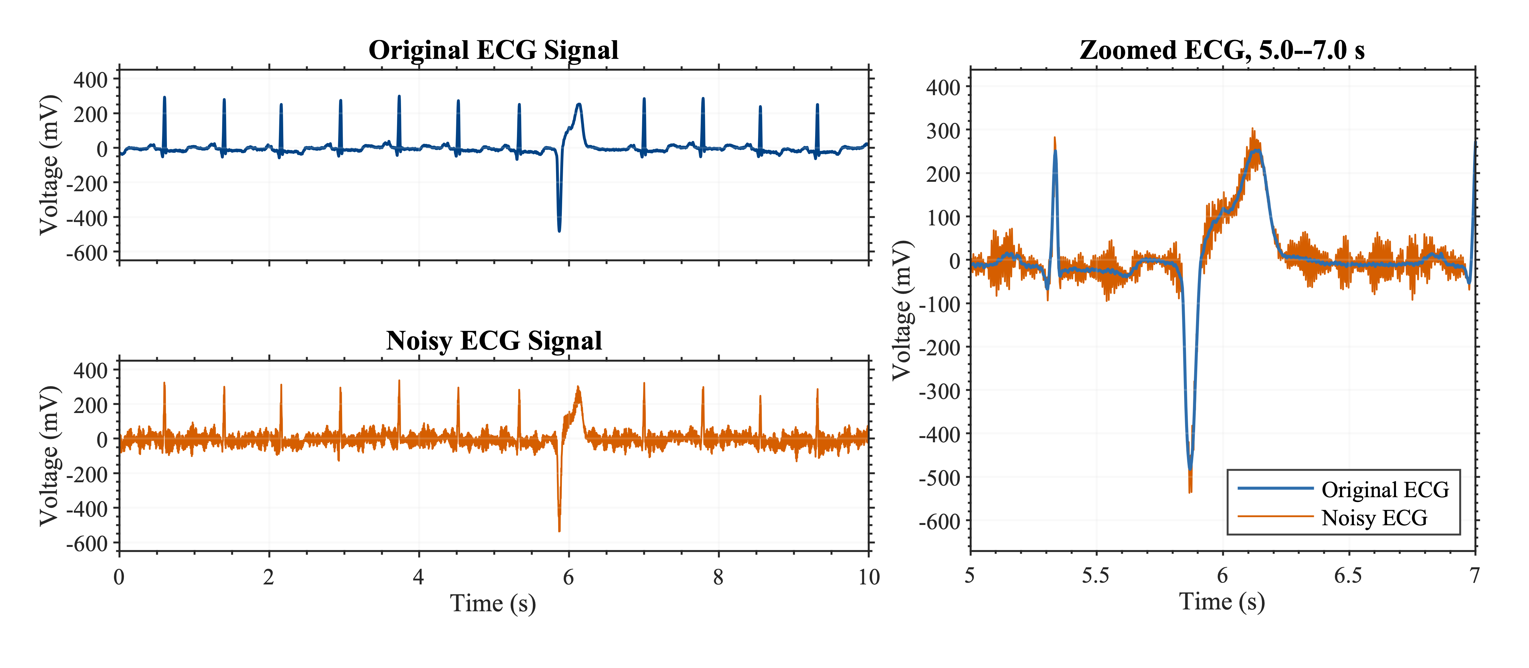
It contains a 10 second ECG recording sampled at 360 Hz, giving 3,600 samples, and includes a clean reference and a corrupted version used for filter evaluation. The record also contains an unusual ventricular waveform around 6 seconds, so simply smoothing the most prominent features would be a poor objective.
The first figure shows how noise thickens the trace, particularly in lower-amplitude regions. The larger QRS deflections remain visible, but visibility alone says little about whether their timing and shape have survived filtering.
I also used a basic peak-detection pass to estimate a nominal heart rate of 72 bpm from 12 detected positive peaks over 10 seconds.
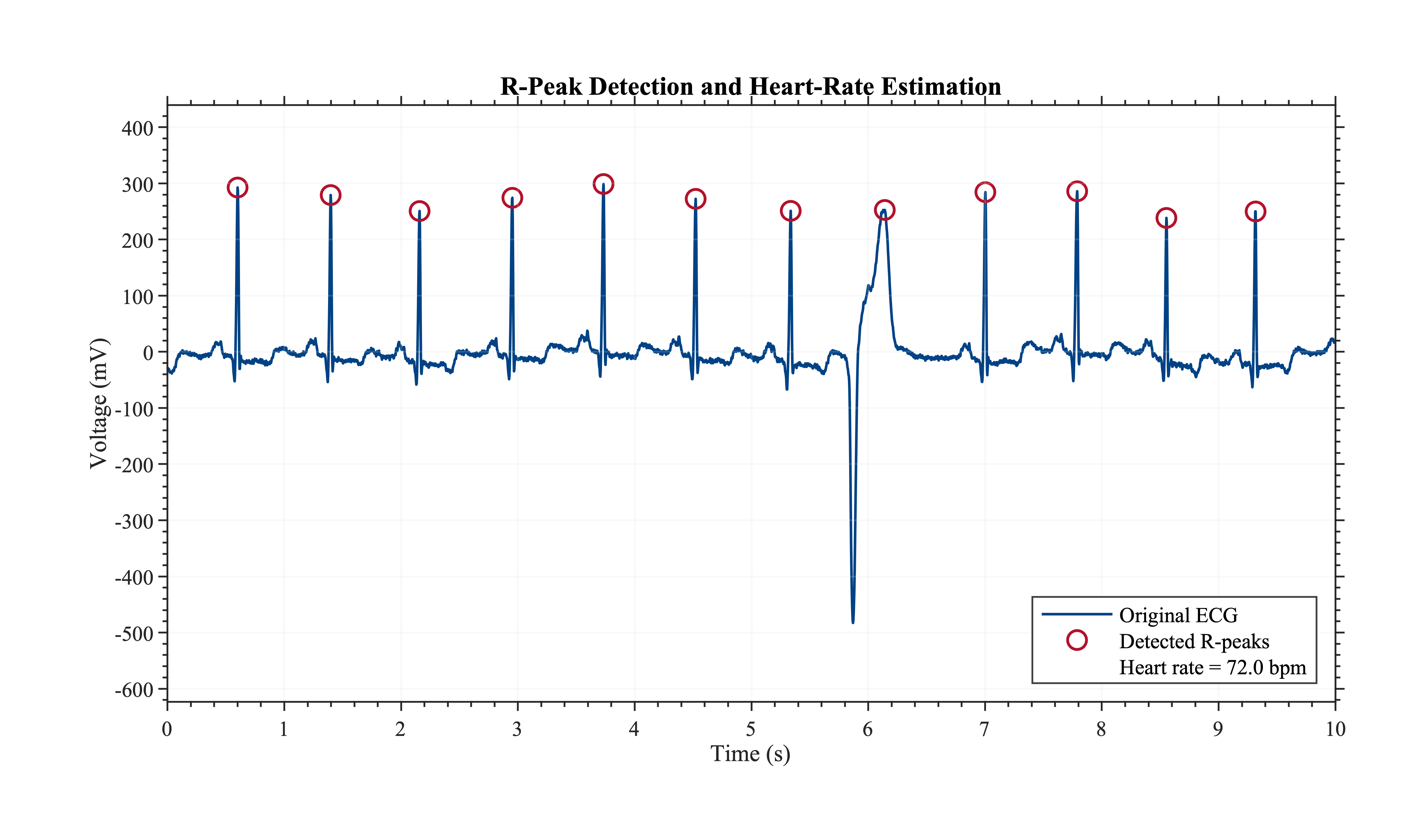
Initial positive-peak detection on the clean reference. The atypical ventricular event illustrates why a simple peak count is not a validated QRS detector or clinical heart-rate assessment.
The peak locations also provided a way to inspect timing changes after filtering. That check is particularly useful when comparing filters with different phase responses.
2. Identify the interference in the frequency domain
Rather than choosing a cutoff from the time-domain trace alone, I inspected the one-sided discrete Fourier transform (DFT) of the noisy recording.
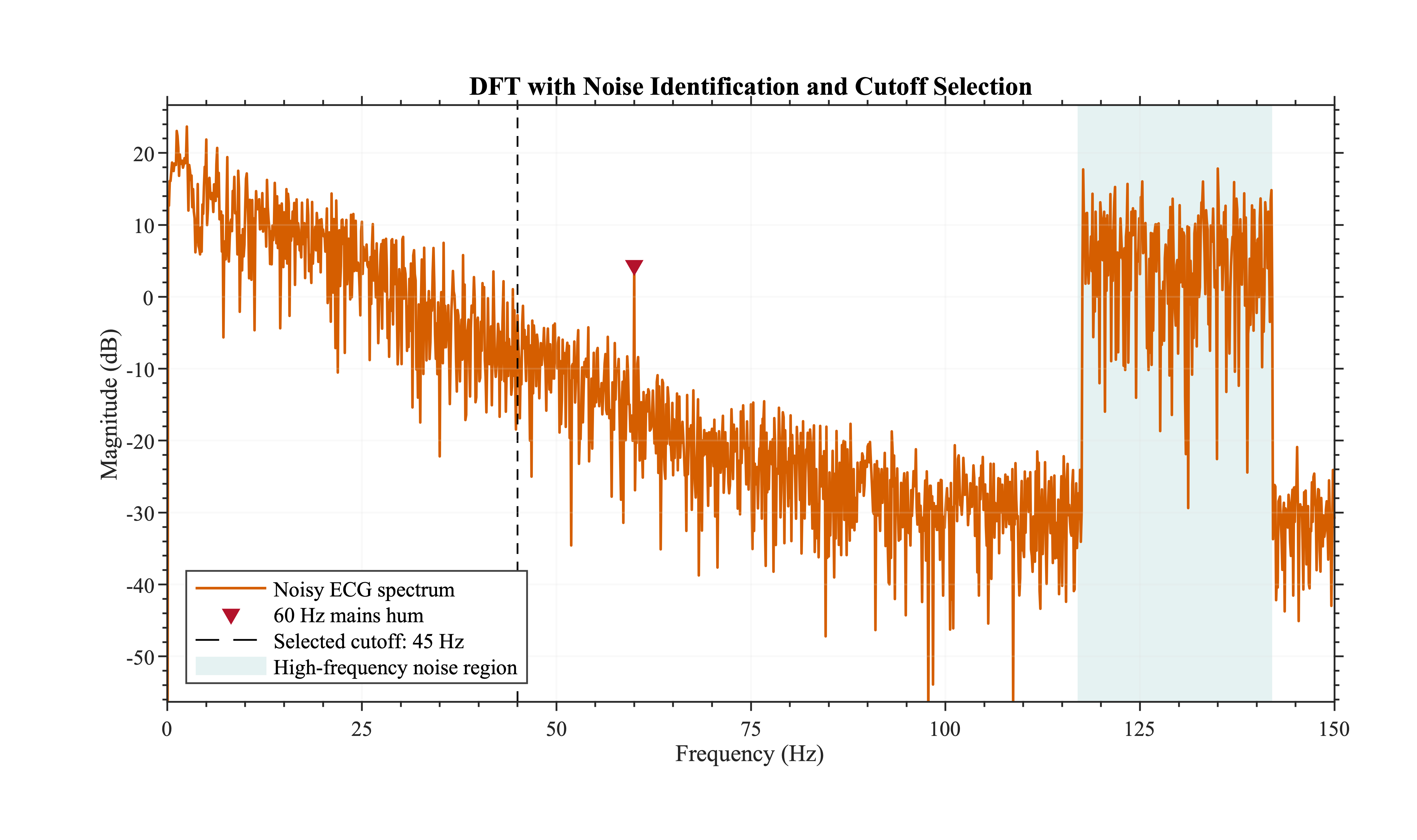
The noisy spectrum contains a narrow component at 60 Hz and a broad elevated band at approximately 117–142 Hz.
These are different interference problems. A narrow spectral component suggests a targeted notch; a broad high-frequency band suggests low-pass attenuation. For the initial comparison, I selected a 45 Hz low-pass cutoff to suppress both components with a single filter.
With a sampling frequency of $f_s=360,\mathrm{Hz}$, the cutoff normalised to the Nyquist frequency is
$$
W_n=\frac{f_c}{f_s/2}=\frac{45}{180}=0.25.
$$
This is a practical first choice rather than a guarantee of optimal waveform preservation. A low-pass filter removes spectral energy according to frequency, not according to whether that energy belongs to interference or to a sharp ECG feature.
3. Two fifth-order filters, two different compromises
The baseline designs used the same nominal order and cutoff:
- FIR: fifth-order low-pass filter designed with a Hamming window.
- IIR: fifth-order Butterworth low-pass filter.
- Common settings: $f_s=360,\mathrm{Hz}$, $f_c=45,\mathrm{Hz}$, applied causally.
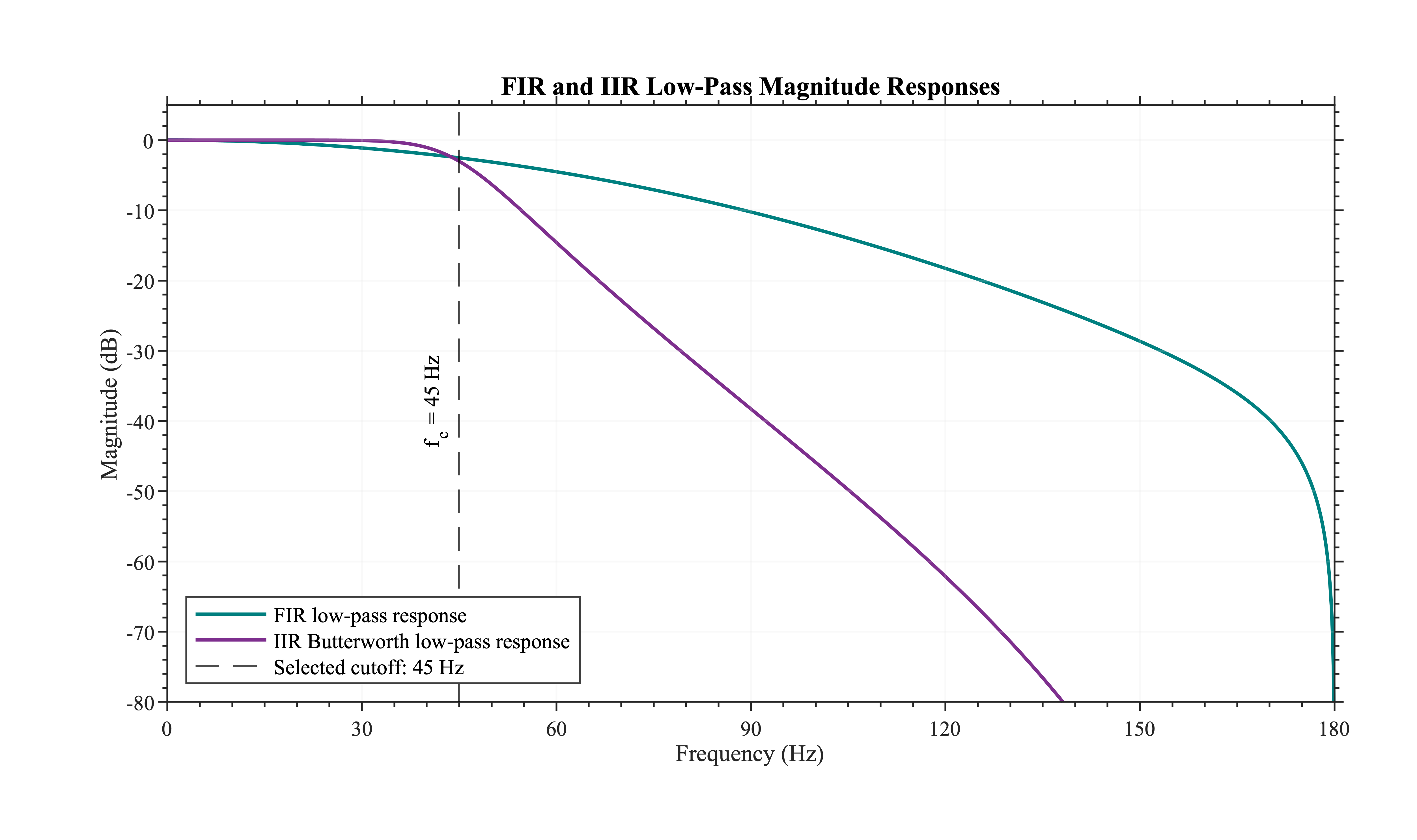
For the same nominal order, the Butterworth IIR gives a much sharper transition. The six-tap FIR attenuates more gradually.
The IIR filter’s frequency response looks more attractive if stopband rejection is the only criterion. Its recursive structure achieves a relatively steep roll-off with a small number of coefficients. The FIR filter is less selective at this short length, but its symmetric coefficients provide linear phase; the waveform is delayed rather than subjected to the IIR’s frequency-dependent phase shift.
Equal order does not mean equal implementation cost or an inherently fair architecture comparison. A fifth-order FIR has six feed-forward taps, whereas the fifth-order IIR uses feedback and has different computational and numerical properties. Here, holding the order fixed was useful for studying behaviour, not for declaring which structure is more hardware-efficient.
4. Cleaner in frequency, less faithful in time
The filtered waveforms exposed the consequence of the different responses.
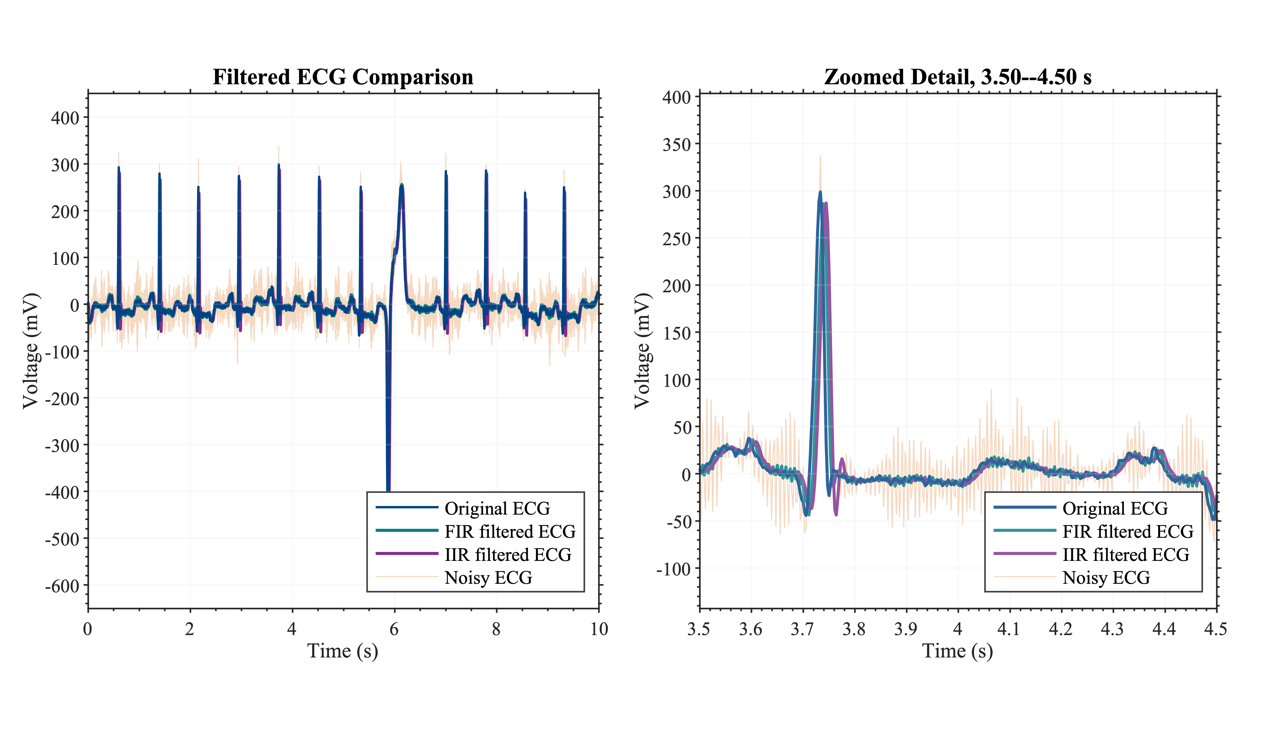
The IIR suppresses more visible noise, but its output is shifted and reshaped around the narrow QRS peak. The FIR retains better alignment with the reference in this example.
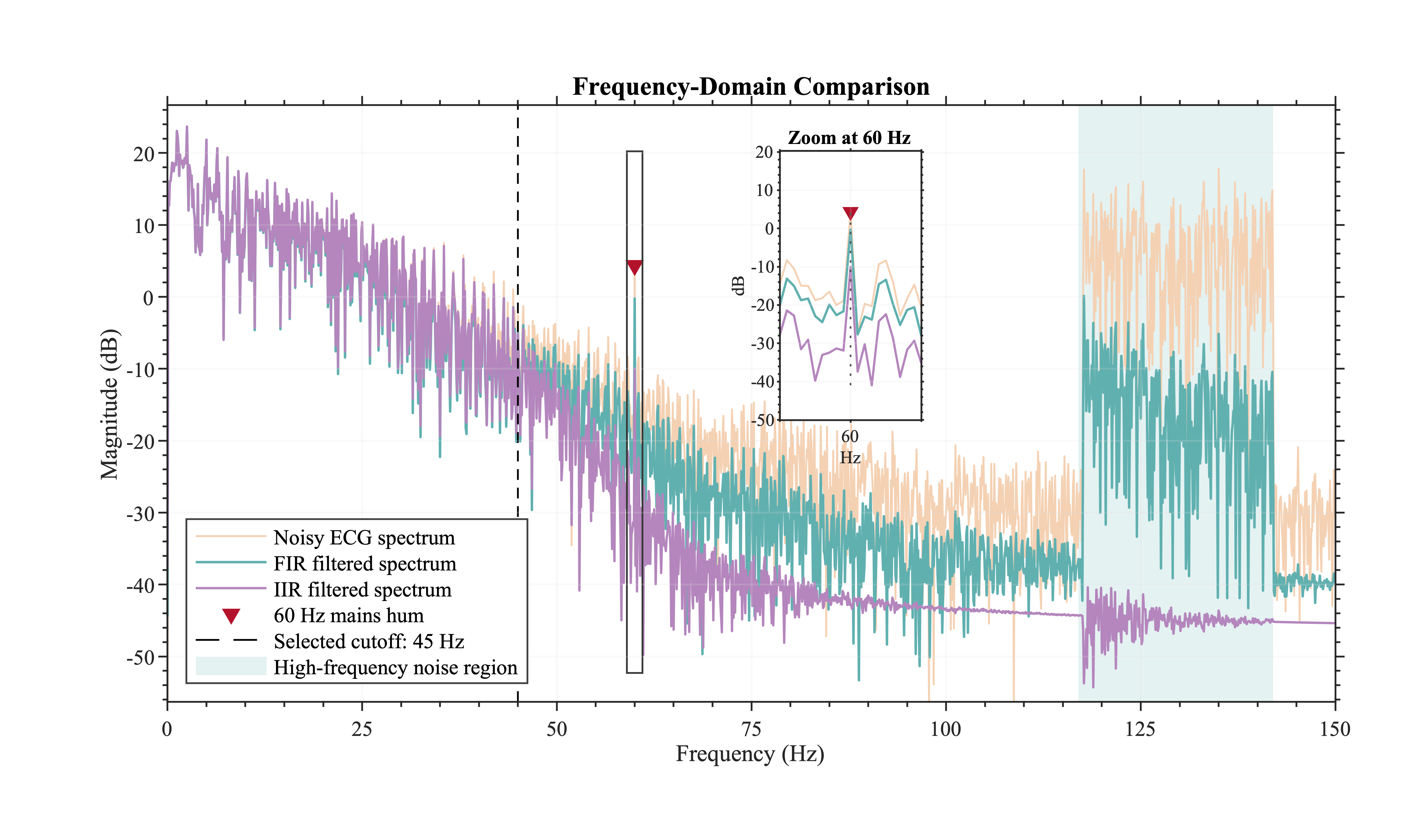
The Butterworth response strongly attenuates the 60 Hz component and the high-frequency band, as expected from its magnitude response.
The quantitative results make the distinction clearer:
| Metric | FIR | IIR |
|---|---|---|
| Overall RMSE (reported mV) | 25.13 | 38.20 |
| Correlation with reference | 0.8873 | 0.7431 |
| SNR improvement (dB) | +1.48 | −2.16 |
| R-peak timing difference (reported ms) | 6.02 | 10.19 |
| 60 Hz reduction (dB) | 4.60 | 14.36 |
| High-frequency reduction (dB) | 21.06 | 51.65 |
The IIR wins on spectral attenuation while losing on reference-based reconstruction metrics. Its greater suppression is not free: it also changes components that contribute to the original waveform. Conversely, the FIR’s smaller reconstruction error does not mean that a six-tap low-pass filter adequately addresses the interference.
That result changed how I approached the next design. Rather than asking one low-pass filter to solve both problems, I separated the narrowband interference from the broader high-frequency noise.
5. A more selective offline filtering strategy
The revised design uses two frequency-selective stages and a different application mode:
| Stage | Configuration | Reason |
|---|---|---|
| 60 Hz notch | Centre: 60 Hz; bandwidth: 2 Hz; $Q\approx30$ | Remove the narrow spectral component without lowering the entire low-pass cutoff |
| Butterworth low-pass | Fifth order; cutoff: 80 Hz | Retain more high-frequency ECG content than the 45 Hz baseline |
| Forward–backward filtering | Zero-phase application of the stages | Avoid net phase delay in offline reconstruction |
The key decision was raising, not lowering, the low-pass cutoff. Once the narrow 60 Hz interference had its own filter, the broader low-pass stage no longer needed to eliminate it by heavily attenuating everything above 45 Hz. The 80 Hz cutoff offers more room for sharp ECG transitions while still reducing the higher-frequency noise band.
Forward–backward filtering removes the net phase delay associated with a single causal pass. It also changes the effective magnitude response, since the signal is filtered in both directions. This matters for interpretation: the revised result benefits from both a different frequency-selective design and a non-causal application method. It is not a controlled comparison of filter topology alone.
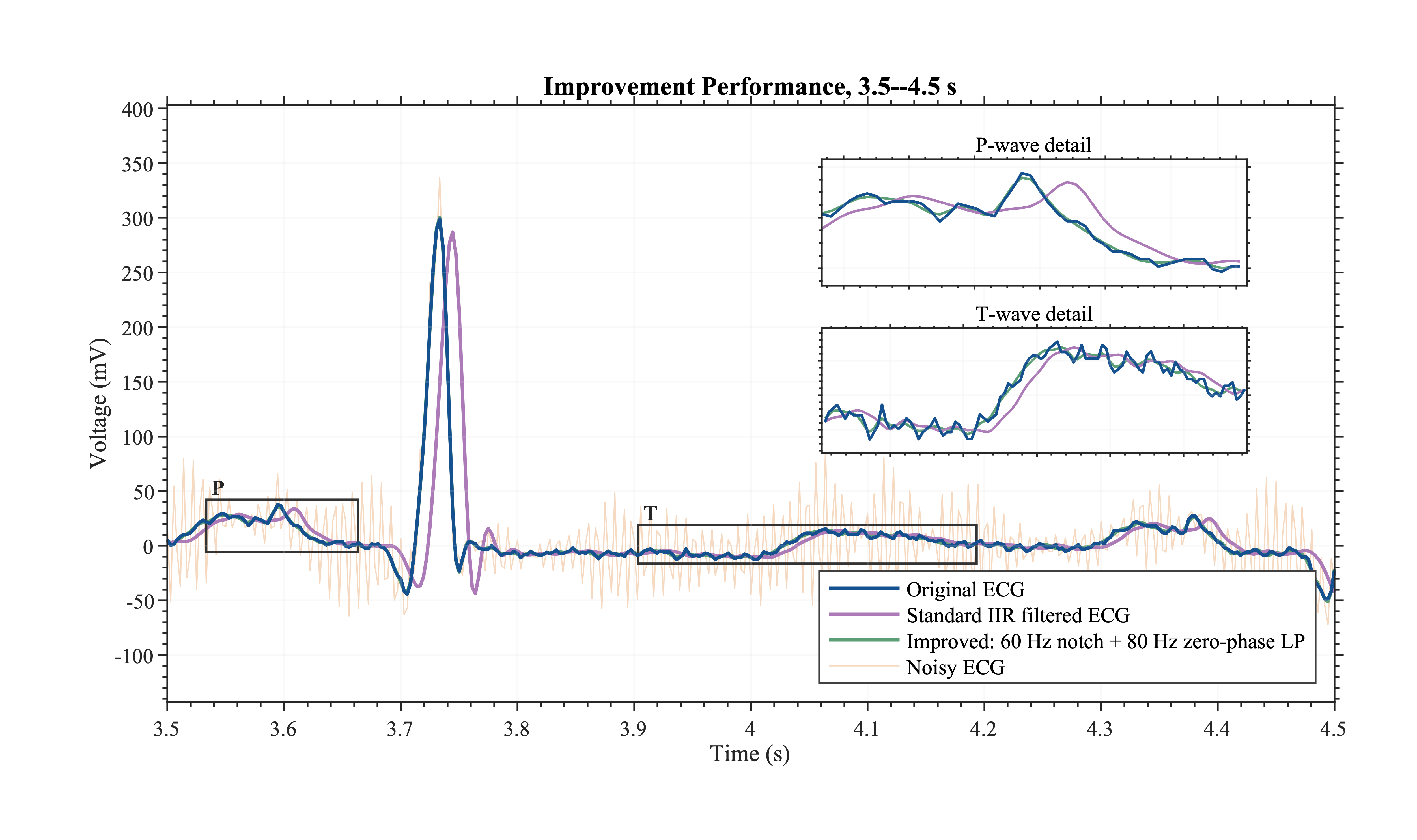
The revised output follows the reference more closely in the selected beat, including the lower-amplitude regions before and after the QRS complex.
6. Results: evaluate reconstruction, not appearance
The final comparison uses RMSE, correlation, SNR improvement, and waveform timing. I also examined local PQRST windows instead of relying only on metrics computed across the entire recording.
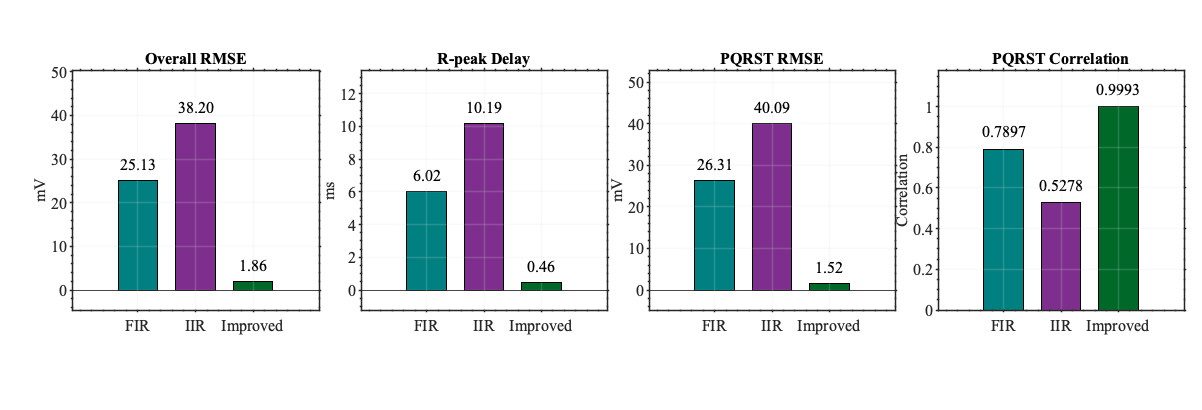
Reported reference-based metrics for the three filter designs on the evaluated 10-second record.
| Metric | FIR | IIR | Revised offline design |
|---|---|---|---|
| Overall RMSE (reported mV) | 25.13 | 38.20 | 1.86 |
| Correlation | 0.8873 | 0.7431 | 0.9994 |
| SNR improvement (dB) | +1.48 | −2.16 | +24.11 |
| R-peak timing difference (reported ms) | 6.02 | 10.19 | 0.46 |
| PQRST-window RMSE (reported mV) | 26.31 | 40.09 | 1.52 |
| PQRST-window correlation | 0.7897 | 0.5278 | 0.9993 |
On this recording, the revised method reduces overall RMSE substantially and raises correlation with the supplied clean signal to 0.9994. The waveform comparison supports the same narrower conclusion: the filtered trace closely follows the reference in the inspected windows.
The timing numbers require care. At 360 Hz, samples are spaced by approximately 2.78 ms. A reported timing difference below one sample interval, such as 0.46 ms, depends on how peak times were estimated and should not be presented as independently demonstrated sub-sample accuracy without checking the measurement code.
7. What’s more?
This was an offline experiment on one 10 second recording, not a validated clinical denoising system. The clean reference makes error measurement possible, but such a reference is generally unavailable when processing a newly recorded ECG. The tested cutoffs also reflect the spectral content of this particular input; robustness across patients, noise levels, and different interference frequencies remains untested.
There is an important implementation boundary as well. Forward–backward filtering needs future samples. A streaming embedded system or FPGA cannot reproduce the same zero-phase result with a straightforward causal pipeline. A real-time version would require an explicit latency budget, causal filter design, and evaluation of fixed-point precision and coefficient quantisation. Its results should be measured separately from this offline benchmark.
I would also recheck the input amplitude calibration and the peak-timing calculations before treating the reported voltage and sub-sample timing figures as physical measurements.
The main lesson from this project was a design one: strong attenuation is a property of a filter, but useful reconstruction is a property of the entire signal-processing task. Frequency-domain analysis helped identify what to suppress; time-domain comparisons and reference-based metrics showed what needed to be preserved. Both views were necessary to make a defensible design choice.