hybrid PI–Residual RL for UAV Motors

A Small, Explainable Patch on Top of PI to improve UAV’s stability and efficiency

This post is a project log of something I personally find more useful than “end-to-end RL replaces classical control”: I kept a conventional PI loop as the stable, interpretable baseline, and added a small, bounded residual correction on top of it. The goal was not to build a huge learning system, but to get a controller that behaves better under realistic nuisances—battery voltage sag, aerodynamic gust disturbances, and ESC-like actuation constraints—while still looking like something I would actually deploy.

The intuition is simple. PI is already doing most of the job. What it often lacks is a lightweight, context-aware correction when the operating conditions shift. Instead of rewriting the controller, I tried to add the missing “last mile” with a residual term that is deliberately limited in magnitude and filtered for smoothness.

Why a hybrid controller instead of pure neural RL

I wanted a controller whose behavior I can reason about and whose failure modes are not mysterious. In UAV motor speed control, the plant is not only nonlinear, but also constrained by very practical effects: duty saturation, duty slew limits, command delay, supply-voltage variations, and short gust-like load disturbances. These are exactly the kinds of details that can make a purely data-driven, high-capacity policy feel overpowered and under-explainable for the problem.

So I treated learning as a controlled add-on. PI remains the main feedback structure. The learned component is only allowed to make a small correction. This gives a clean engineering story: the baseline loop dynamics are preserved, while the residual absorbs some modeling mismatch and disturbance-induced transient issues.

The setup: make “realism” part of the simulation

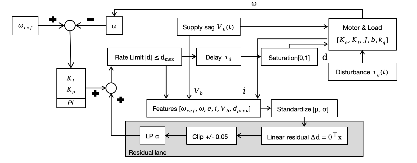
The simulation includes (i) a supply-voltage sag model to reflect a 3S battery droop over short horizons, (ii) a gust disturbance modeled as a short Gaussian torque pulse, and (iii) ESC-like actuation constraints: PWM duty in $[0,1]$, a duty rate limit, and a fixed command delay. The point is not to perfectly model every electrochemical detail, but to ensure the controller is trained and evaluated in conditions that resemble how a motor actually feels inside a UAV.

The reference is intentionally hybrid (ramp + steps + sinusoids) so the controller is forced to handle startup, tracking, and small oscillatory components in a single episode, while the gust creates an obvious transient “stress test” segment.

Control structure: PI baseline + bounded linear residual

The controller can be summarized as:

$$
d(t) = \mathrm{sat}\big(d_{\mathrm{PI}}(t) + \Delta d(s),, 0,, 1\big)
$$

The residual policy is deliberately simple and explainable: it is a linear mapping from a normalized state vector to a duty-cycle correction, followed by a hard clip:

$$
\Delta d(s) = \mathrm{clip}(\theta^\top s,,-a_{\max},,a_{\max})
$$

The state vector contains the instantaneous speed error, the integral error, the measured motor current, and the supply voltage. The residual output is additionally low-pass filtered before being applied, which reduces high-frequency switching and keeps the correction “well-behaved” even when the PI loop is already close to steady state.

The key design choice is that the residual is not allowed to dominate. With a small correction bound, saturation, and actuator constraints, the residual behaves like a patch—not a second controller fighting the first one.

Training without drama: random search and multi-objective selection

Because the system includes saturation, slew limiting, and delay, I avoided making this a “big RL pipeline” problem. Instead, I optimized the residual parameters $\theta$ offline using a gradient-free random search: propose candidate parameters, simulate a full episode, score performance, and iterate.

The objective is multi-criteria by design. Each rollout logs:

$$
\text{Tracking} \rightarrow \text{ITAE}, \qquad
\text{Energy} \rightarrow E_{\mathrm{Wh}}, \qquad
\text{Smoothness} \rightarrow \text{BandPow}_{lf}
$$

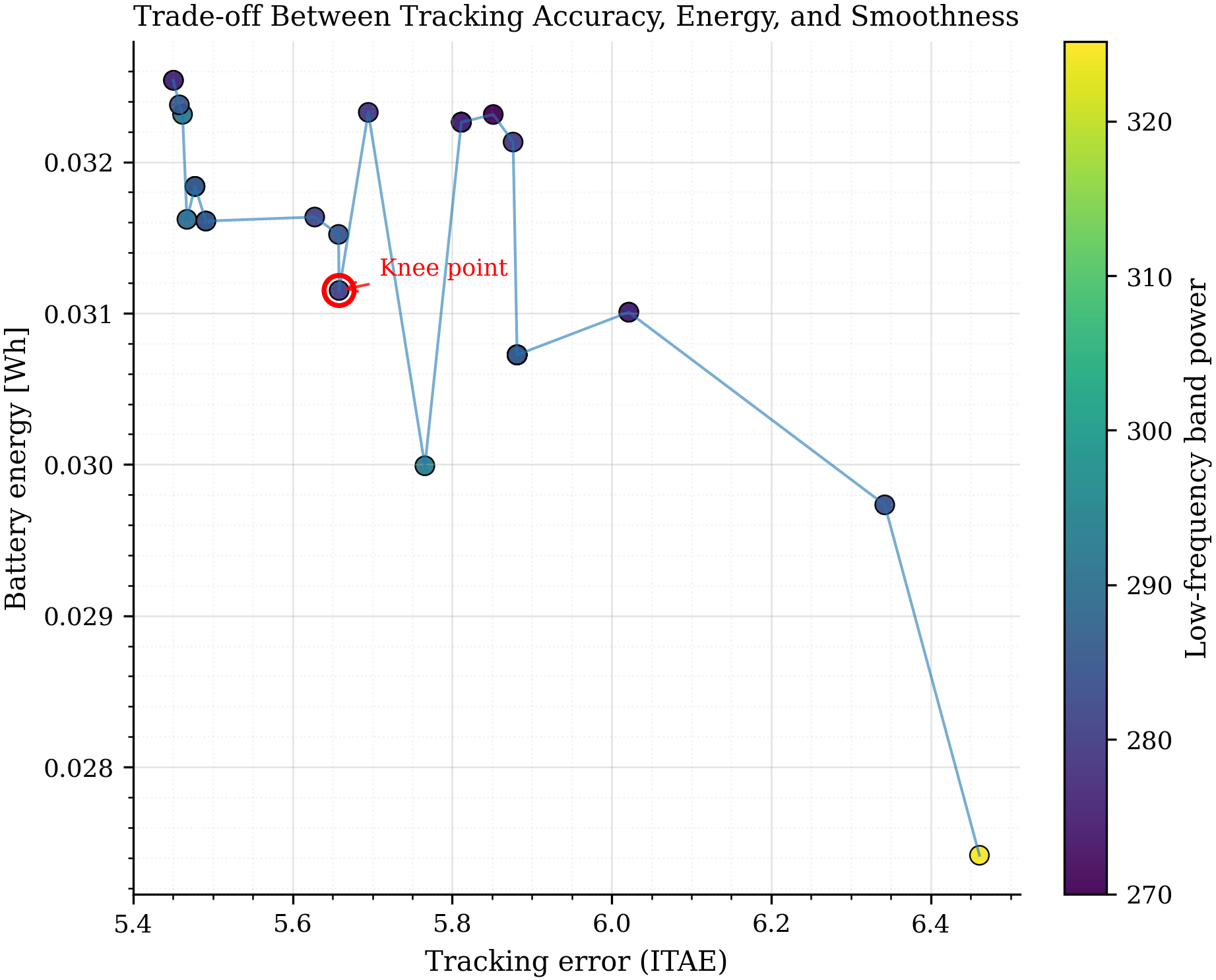
Rather than forcing a single weighted sum to decide everything, I treated the results as a Pareto trade-off surface and used hypervolume-based selection to identify a balanced controller. This matters because it is easy to reduce ITAE further by becoming more aggressive, but doing so can increase current draw and degrade smoothness without meaningful steady-state benefits.

Results: better transient behavior where it matters

The plot below compares the reference, the pure PI baseline, and the hybrid controller. The “gust region” is the part that tends to expose whether a controller can reject disturbances cleanly without creating long, low-frequency oscillations. What I wanted from the residual is not magical tracking in every segment, but a more controlled transient: less lingering oscillation and a more decisive recovery.

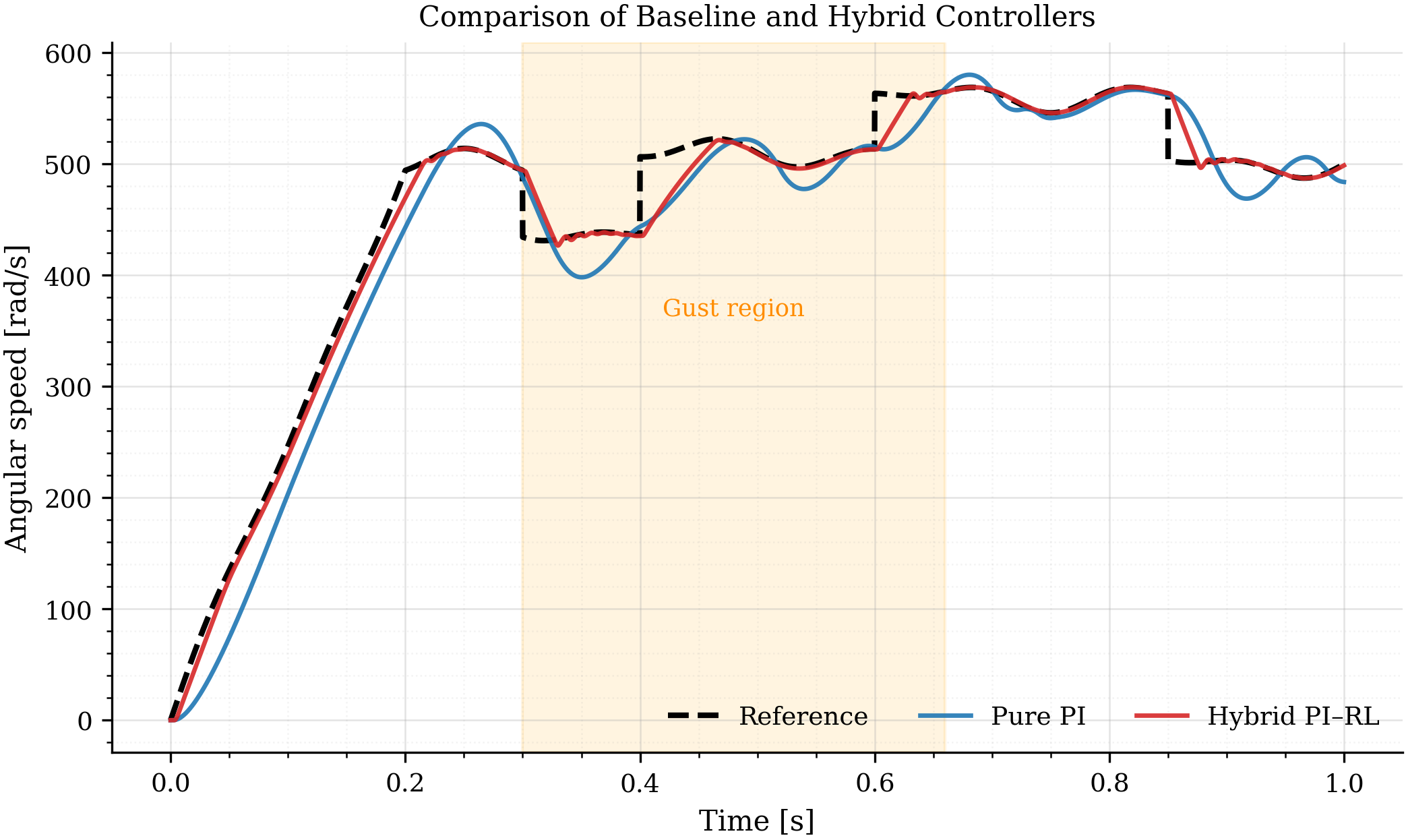
Quantitatively, the knee-point hybrid setting improves ITAE and the low-frequency band-power metric substantially compared to the PI baseline, with a small energy trade-off. In my run, ITAE drops from 12.427 to 5.628 and $\text{BandPow}_{lf}$ drops from 731.873 to 281.221, while energy increases from 0.030 Wh to 0.032 Wh. This is the kind of exchange I consider “engineering plausible”: a mild energy increase to buy a much cleaner dynamic response.

Why I picked the knee point (and not the “best ITAE” point)

Once you see the Pareto front, it becomes obvious that chasing only accuracy is not free. You can push ITAE down further, but you start paying with slightly higher energy and, depending on the setting, less desirable smoothness. In other words, past a certain point the marginal gain in tracking is not worth the added aggressiveness.

The knee point is a pragmatic default. It is not the extreme “accuracy-only” controller, and it is not the “energy-only” controller. It is the place where you still get most of the tracking and smoothness benefits without taking the full cost.

Why this looks deployable (to me)

The online computation is tiny: a dot product, a clip, and a first-order low-pass filter. There is no neural network inference and no complex memory state to manage. More importantly, the structure stays interpretable. If the controller changes behavior, there is a concise place to look: the residual weights $\theta$, and the state channels that drive them.

The safety story is also straightforward: the residual amplitude is bounded; the final duty is saturated; the command is rate-limited; and the actuation delay is explicitly modeled. In practical terms, the residual is prevented from “doing something clever” that a real ESC could never execute.

Reproducibility notes and next steps

Each episode runs for 1.0 s with sampling interval $dt = 2 \times 10^{-4}$ s. The duty rate limit is $8~\mathrm{s}^{-1}$, the ESC command delay is 2 ms, the residual clip is $\pm 0.05$, and the residual low-pass coefficient is $\alpha = 0.6$. PI gains are fixed; only $\theta$ is optimized offline.

Next, I want to move beyond a single-motor setup. Multi-motor propulsion introduces coupling and shared supply dynamics that could make the residual either more valuable or more sensitive. I also want to test the same hybrid idea under sensor noise, quantization, and communication delays, because those are the details that tend to decide whether a “good simulation controller” becomes a practical controller.

If you are also interested in the “classical control + tiny learning patch” direction, I think this is a promising pattern: keep the proven feedback structure, and use learning only where it has the highest leverage.