Pipelined INT8 Vector MAC on FPGA

Wallace Tree, Scaling, and the Real Cost of “Fast”

At a glance, the Wallace tree looks like an elegant hack: take a tall matrix of partial products and squash it into two rows quickly, then finish with a normal carry-propagate adder. What becomes more interesting in practice is that Wallace is not simply “faster multiplication”. It is a statement about where you want complexity to live. Instead of letting carries ripple all the way across at every intermediate addition, you keep carries local by using carry-save compression (3:2 compressors, i.e., full adders) until the very end. In other words, Wallace postpones global carry resolution and spends area and routing to buy down logic depth. On an FPGA, that trade is never purely logical; it is also physical. The structure you choose shapes the placement and wiring, which can matter as much as the gate-level critical path.

Worst-case sizing as a first-class constraint

Before discussing clocks and lanes, the arithmetic bound has to be explicit. With unsigned INT8 operands, the maximum product is

$$
P_{\max} = 255 \times 255 = 65025 = 2^{16} - 511.
$$

This single number governs the widths of the multiplier output, the adder tree, and the accumulator. The objective here is not to minimise bitwidth at all costs; it is to choose widths that are safe, structurally consistent across $N$, and convenient for pipelining.

Block	Operand range	Max. output	Chosen width	Latency
8×8 Wallace multiplier	$(0 \ldots 255)$	$(255^2 = 65025)$	17-bit	3 stages
Adder tree $(N = 1\text{–}16)$	$(N)$ products	$(N \times 65025)$	20 bit (at $N=16$)	$\max(2,\lceil \log_2 N \rceil)$
Accumulator (up to 1000 beats)	dot products	$(1000 \times 65025)$	32-bit	1 cycle

There are three decisions embedded in Table I that are easy to miss if you only look at the final RTL. First, the multiplier output is carried on 17 bits. While $65025$ fits in 16 bits, the additional guard bit makes the reduction and final CPA less fragile, especially when the multiplier is deeply pipelined and internal carries are being staged. Second, the adder tree width is driven by the worst-case merge of $N$ products, with the upper bound

$$
S_{\max}(N) = N \cdot 65025,
$$

and the tree depth is treated as a structural parameter rather than an afterthought,

$$
L_{\text{tree}}(N) = \max(2,\lceil \log_2 N \rceil).
$$

Third, the accumulator is kept at 32 bits even though $1000 \times 65025 = 65{,}025{,}000$ would fit in fewer bits. On FPGA, 32-bit arithmetic is a comfortable “native” size that simplifies integration, and it gives headroom for extending the design (wider operands, higher beat counts) without reopening every bound.

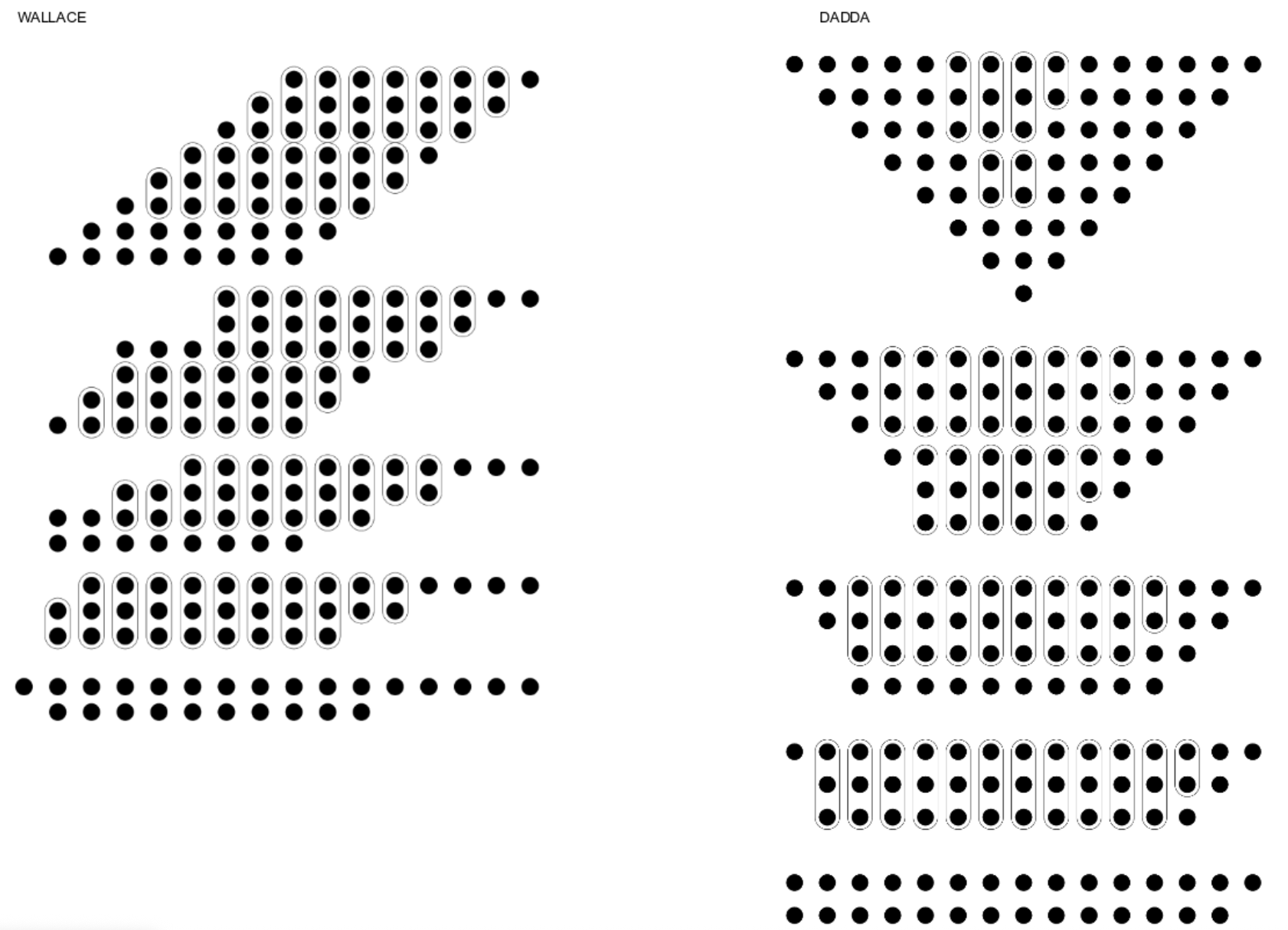
What the Wallace tree is actually buying

The Wallace tree is best described as a parallel reduction scheme for partial products. An $8\times 8$ multiplier generates eight shifted rows of partial products. If you add them naively, you either do it sequentially (shift-add over multiple cycles) or you build an array-like reduction where carries propagate repeatedly across the width. Wallace changes the game by using 3:2 compression to reduce the height of the matrix quickly without propagating carries globally at each step.

The practical effect is that the “hard” part of the computation is reorganised into a sequence of local operations. Each compression layer shortens the vertical dimension of the bit matrix and only emits carries to the next higher-weight column. This is why Wallace trees pair naturally with pipelining: you can register between compression layers and keep the combinational depth under control. The final CPA is the only place where full carry propagation is allowed to happen.

The less romantic part is that on FPGA, the “local” nature of compression is not guaranteed to be local in placement. A Wallace tree produces a dense pattern of adders with a wide fan-in/fan-out across adjacent bit columns. With small widths like 8×8 this is manageable, but once you replicate lanes and add a pipelined adder tree on top, routing becomes a real cost centre. This is the main reason I did not treat “Wallace tree = fastest” as a blanket truth; instead, I treated it as a design choice whose value must be validated post-implementation, not just post-synthesis.

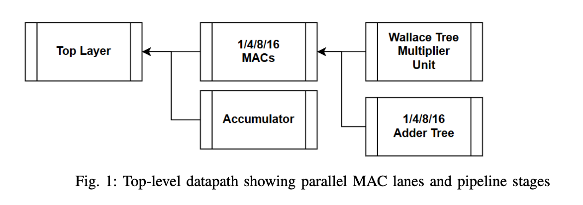
Pipeline structure and a latency model that stays simple

The multiplier is implemented as a three-stage pipelined Wallace reduction, followed by a final carry-propagate addition. Lane merging is done with a registered binary adder tree whose depth scales with $\log_2 N$. The accumulator adds one more registered stage under beat control. With this structure, the total latency remains predictable and the initiation interval stays at one cycle once the pipeline is filled. A simple mental model for the end-to-end latency in cycles is

$$
L_{\text{total}}(N) \approx 3 + \log_2(N) + 1,
$$

where the first term is the multiplier pipeline depth, the second term is the merging tree depth, and the final term is the accumulator stage. This is not meant to be a formal proof; it is meant to keep the design composable. When $N$ changes, the story does not change, only the constants do.

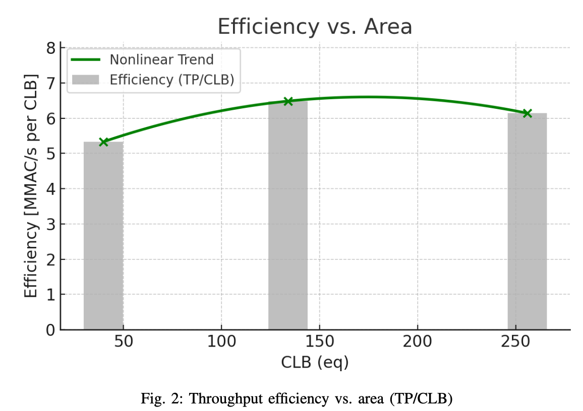
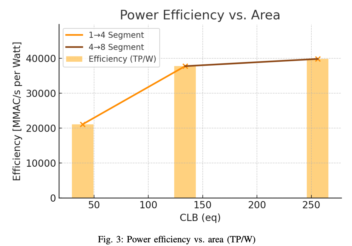
Post-implementation results: where scaling is “worth it”

After implementation, I compared configurations using an effective throughput definition

$$
TP = \text{Lanes} \times F_{\max},
$$

and then normalised it both by area (CLBeq) and by power. The point here is to make scaling effects visible. If $N$ doubles but $F_{\max}$ collapses, the architectural decision is not actually buying throughput.

Config	Latency [ns]	CLBeq	$F_{\max}$ [MHz]	Power [W]	$TP$	$TP/\text{CLB}$	$TP/W$
1×8×8	4.736	39.6	211	0.010	211	5.33	21.1
4×8×8	4.603	133.85	217	0.023	868	6.49	37.7
8×8×8	4.780	285.85	209	0.042	1672	6.23	39.8

The most useful conclusion from Table III is that scaling is not monotonic in “goodness”. The 4-lane configuration delivers the best throughput per area, which is a strong indicator that it sits near the efficient knee of this design’s scaling curve. The 8-lane configuration leads throughput per watt, which is consistent with amortising shared overheads, but it gives up some area efficiency, and it is also the most exposed to routing pressure. That observation is aligned with the earlier Wallace-tree reflection: once the design becomes physically dense, timing and power are no longer driven only by logical depth. They are driven by how hard the placer/router has to work to keep high-activity signals short and well-clustered.

A more honest takeaway on Wallace trees

If I had to compress the Wallace-tree lesson into one sentence, it would be this: Wallace is a technique for trading carry propagation depth for compressor density, and on FPGA that trade is mediated by routing. In small multipliers, Wallace often “just works” and gives you a clean pipelinable core. In a scalable lane-based design, Wallace becomes one of several interacting structures that collectively decide whether the design is compute-bound or wire-bound.

In this project, pipelining the Wallace reduction into three stages was not merely about increasing $F_{\max}$. It was about making the multiplier’s internal carry-save representation explicit and stageable, so that the rest of the system—lane replication, tree merging, accumulation—can be reasoned about with stable interfaces. The bigger win is architectural hygiene: once the multiplier is a well-behaved, latency-known component, the rest of the datapath can be tuned and scaled without repeatedly re-solving the same timing puzzle.

If I extend this work, the most interesting direction is not to add more lanes blindly, but to treat physical locality as a design parameter: clustering lanes, shaping the adder tree to match placement, and possibly exploring alternative compressor schedules that map more naturally onto FPGA fast-carry resources. That is the point where “multiplier architecture” stops being an isolated block choice and starts being full-stack hardware design.

Code

Source code available: https://github.com/0xCapy/Vector-multiplier.git

---